A few facts about Flow Matching

Fact-1: There are three different types of $x_0$. (#)

Fact-2: The inference time ODE is curved. (#)

Fact-3: For real datasets, $\mathbb{E}[x_0\mid x_t]$ follows Softmax-weighting. (#)

Fact-4: $x_0^{\text{ODE}}$ and $x_0^{(i)}$ have the same marginal distribution. (#)

Fact-1: Three Different Types of $x_0$

There are 3 different types of $x_0$: the training sample $x_0^{(i)}$, the conditional expectation $\mathbb{E}[x_0\mid x_t]$, and the ODE endpoint $x_0^{\text{ODE}}$. These three are generally not the same points.

Below we use a counterexample to show why these 3 are different.

Setup. Noise $x_1\sim \mathcal{N}(0,1)$, clean data $x_0\sim \mathcal{N}(\mu ,{\sigma }_0^2)$, , and interpolation:

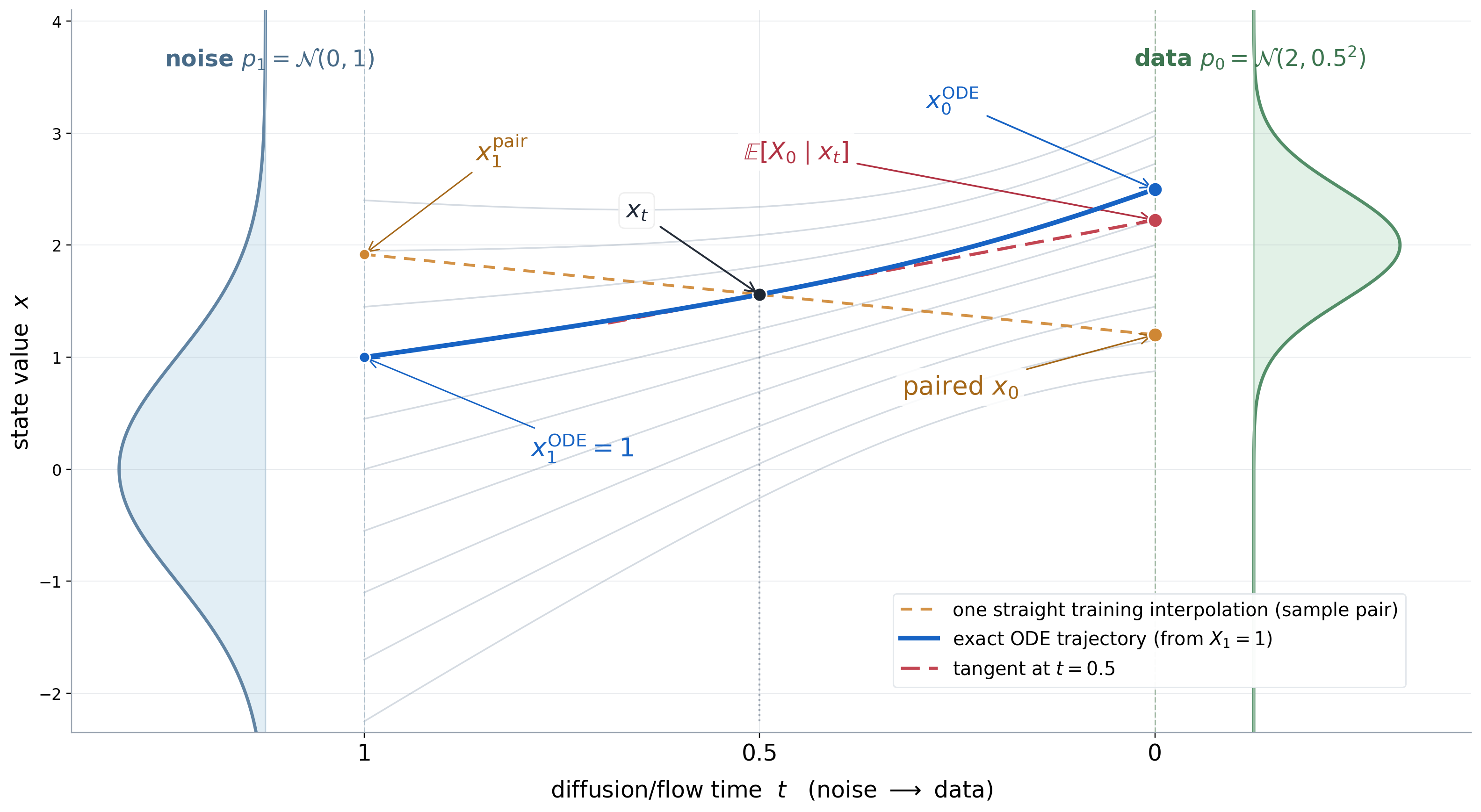
A visual example. The plot below visually compares these three types of $x_0$. The brown $x_0$ is paired with $x_1^{\text{pair}}$, their interpolation is $x_t$. These are used for training. But the learnt velocity (tangent) at $x_t$ points at the pink $E[X_0|x_t]$. And even the tagent itself is changing along $t$, where at ODE terminal the actual endpoint is the blue $x_0^{\text{ODE}}$.

Below is a derivation of these three $x_0$.

1. Marginal Distribution $p(x_t)$.

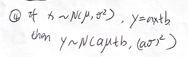
First let us check the marginal $p(x_t)$. Making use of the(my) probability tool, we treat $x_1$ as noise, and $t{x}_1\sim \mathcal{N}(0,t^2)$ because of the Formula-4 below,

Then we use Formula-9,

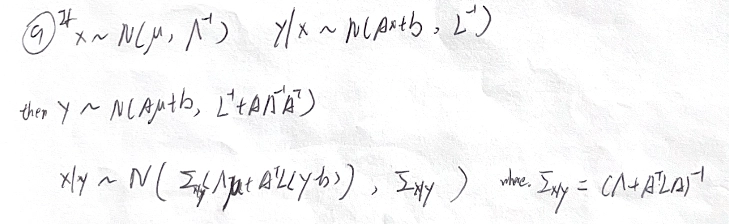
more specifically,

• Let $x_0$ be $X$, with ${\mu }_X=\mu$ and ${\Lambda }^{-1}={\sigma }_0^2$.

• Let $x_t$ be $Y$. Since $x_t=(1-t)x_0+t{x}_1$, we have $A=1-t$, $b=0$, and $L^{-1}=t^2$.

Checking Formula-9’s Line-2, that $Y\sim N(A{\mu }_X+b,A{\Lambda }^{-1}{A}^T)$, where $A{\mu }_X+b=(1-t)\mu$, and $L^{-1}+A{\Lambda }^{-1}{A}^T=t^2+(1-t{)}^2{\sigma }_0^2$. This leads to the marginal distribution of $x_t$,

(Note: we could also have used the stacked vector $(x_0,x_1{)}^T$, but later finding the posterior $x_0\mid x_t$ would be annoying).

2. Conditional Expectation $\mathbb{E}[x_0\mid x_t]$

Secondly, we find $\mathbb{E}[x_0\mid x_t]$. By Line-3 in Formula-9:

Combining above two to find the mean, we get:

For convenience, we introduce the marginal variance ${\sigma }_t^2=t^2+(1-t{)}^2{\sigma }_0^2$, so equivalently:

3. ODE Endpoint $x_0^{\text{ODE}}$

Thirdly, we find the ODE endpoint. To do so, we will follow the ODE using the learnt velocity. At training time, the velocity objective minimises ${\mathbb{E}}_{x_0,x_t}\left[{\Vert \hat{v}(x_t,t)-\frac{d{x}_t}{dt}\Vert }_2^2|x_t,t\right]$, whose minimiser is ${\hat{v}}^{\ast }(x_t,t)=\mathbb{E}\left[\frac{d{x}_t}{dt}|x_t,t\right]$.

By the definition of $x_t$, where we again treat $x_1$ as the noise of $x_t$,

Thus:

Plugging in $\mathbb{E}[x_0\mid x_t]$, we get a (seemingly complicated) velocity:

Solving the toy ODE. We need to solve $\frac{d{x}_t}{dt}={\hat{v}}^{\ast }(x_t,t)$; the solution of this ODE at $t=0$ will give us the endpoint $x_0^{\text{ODE}}$.

We use a (Chatgpt provided) trick by introducing $z=x_t-(1-t)\mu$, hence $x_t=z+(1-t)\mu$. After rearranging, the RHS becomes $-\mu +\frac{t-(1-t){\sigma }_0^2}{{\sigma }_t^2}z$, and the LHS is $\frac{d{x}_t}{dt}=\frac{dz}{dt}-\mu$. Cancelling $\mu$ on both sides yields:

From here, we move $dt$ to the RHS and move $z$ to the LHS.
For the RHS, we further introduce $u(t)={\sigma }_t^2=t^2+(1-t{)}^2{\sigma }_0^2$, because $\frac{1}{2}\frac{du(t)}{dt}=[t-(1-t){\sigma }_0^2]$, which is the numerator.
The RHS is thus $\frac{\frac{1}{2}\frac{du(t)}{dt}}{u(t)}dt=\frac{1}{u(t)}du(t)$, which leads to the following simplified ODE,

Taking the definite integral ${\int }_{z(t)}^{z(0)}\frac{2}{z}dz={\int }_{u(t)}^{u(0)}\frac{1}{u}du$, we get:

Substituting the boundary values,
$u(0)={\sigma }_0^2$, $u(t)={\sigma }_t^2$, $z(0)=x_0^{\text{ODE}}-\mu$, and $z(t)=x_t-(1-t)\mu$:

4. Final Comparison

If we rearrange $\mathbb{E}[x_0\mid x_t]$ by replacing $t^2={\sigma }_t^2-(1-t{)}^2{\sigma }_0^2$, we get:

Comparing $x_0^{\text{ODE}}$ and $\mathbb{E}[x_0\mid x_t]$, we see that they have different scaling factors ($\frac{{\sigma }_0}{{\sigma }_t}$ vs. $\frac{(1-t){\sigma }_0^2}{{\sigma }_t^2}$) and are not the same, completing the proof of the counterexample.

Fact-2: The inference time ODE is curved.

This is obvious from the above example.

Fact-3: For real datasets, $\mathbb{E}[x_0\mid x_t]$ follows Softmax-weighting.

In Fact-1, we used a simplified clean data distribution to demonstrate how three types of $x_0$ are different. For real datasets, we do not have the nice Gaussian posterior property anymore (Formula-9), but we can still use Bayes’ theorem to derive $\mathbb{E}[x_0\mid x_t]$.

Setup. $x_0$ now follows the real data distribution $p_{\text{data}}(x_0)$, while $x_1\sim \mathcal{N}(0,I)$ still. There are two cases to consider: the theoretical case where $p_{\text{data}}(x_0)$ is continuous, and the empirical case where $p_{\text{data}}$ is discrete.

The theoretical continuous $p_{\text{data}}(x_0)$

We start by writing:

By Bayes’ theorem:

Next, we show that:

To see this, note that:

Note that $p(x_t\mid x_1,x_0)$ is $\infty$ (integrating to $1$) only at $x_t=t{x}_1+(1-t)x_0$, and is $0$ elsewhere when $x_t\ne t{x}_1+(1-t)x_0$. So $p(x_t\mid x_1,x_0)=\delta (x_t-[t{x}_1+(1-t)x_0])$.

Introducing $u=t{x}_1+(1-t)x_0⟹x_1=\frac{u-(1-t)x_0}{t}$ and $d{x}_1=\frac{1}{t^D}du$ (where $D$ is for the $D$-dim Jacobian determinant), the integral becomes:

where $p_{x_1}$ follows $\mathcal{N}(0,I)$, which gives the exp-square term.

Going back to $p(x_0\mid x_t)$, we have:

Let the normalised probability be $p(x_0\mid x_t)=\frac{1}{Z}\frac{1}{t^D}\exp \left(-\frac{\Vert x_t-(1-t)x_0{\Vert }^2}{2t^2}\right)p_{\text{data}}(x_0)$.
Since:

we get $Z=\frac{1}{t^D}\int \exp \left(-\frac{\Vert x_t-(1-t)x_0^{\prime }{\Vert }^2}{2t^2}\right)p_{\text{data}}(x_0^{\prime })d{x}_0^{\prime }$. Hence, the $\frac{1}{t^D}$ cancels out:

where $C=\int \exp \left(-\frac{\Vert x_t-(1-t)x_0^{\prime }{\Vert }^2}{2t^2}\right)p_{\text{data}}(x_0^{\prime })d{x}_0^{\prime }$.

Therefore,

The real discrete $p_{\text{data}}(x_0)$

The above $\mathbb{E}[x_0\mid x_t]$ is also true for the discrete case. However, since a practical dataset has a finite number of $N$ samples $\{x_0^{(1)},\dots ,x_0^{(N)}\}$ and each sample $x_0^{(i)}$ is picked uniformly, $p_{\text{data}}(x_0^{(i)})=\frac{1}{N}$ and $p(x_0\mid x_t)$ is $0$ elsewhere.

The normalising constant $C$ for the posterior $p(x_0^{(i)}\mid x_t)$ is now a sum over the $N$ samples, and $\frac{1}{N}$ cancels out:

Again, $p(x_0\mid x_t)=0$ for $x_0\ne x_0^{(i)}$. Thus:

We can analyse this empirical $\mathbb{E}[x_0\mid x_t]$ across time $t$:

• At $t\to 1$: Since $(1-t)x_0^{(i)}=0$, the term ${\text{Softmax}}_i(\dots )$ is the same ($\frac{1}{N}$) for every sample $i$, so $\mathbb{E}[x_0\mid x_t]$ points to the global average of $x_0^{(i)}$ across the dataset.

• At $t\to 0$: The Softmax term $\to \text{argmax}$, and $\mathbb{E}[x_0\mid x_t]\to x_0^{(i^{\prime })}$ at the particular sample $x_0^{(i^{\prime })}$ that has the smallest (nearest) distance $\Vert x_t-x_0^{(i)}{\Vert }^2$. So the velocity points to a single specific training sample $x_0^{(i^{\prime })}$.

• At $0<t<1$: Here $2t^2$ acts as the Softmax temperature evolving the smoothing radius along $t$; $\mathbb{E}[x_0\mid x_t]$ points to a local weighted average of nearby samples. As $t$ decreases, these weights shift continuously from the global mean $\to$ local clusters $\to$ a single sample, causing the ODE velocity to constantly change direction.

This concludes the fact of Softmax-weighting for the empirical case in real datasets. The above analysis also explains why the inference-time ODE trajectory is curved.

Q: Does the above mean Flow Matching cannot generate new samples unseen from the dataset? Mathematically, yes. As we see above, the exact empirical Softmax solution turns into a hard argmax as $t\to 0$, which memorises the dataset. In practice, Flow Matching generates novel samples because the neural network learnt velocity fields do not exactly reproduce the optimal velocity field, and the corresponding ODE’s endpoint can deviate from the training samples.

Fact-4: $x_0^{\text{ODE}}$ and $x_0^{(i)}$ have the same marginal distribution

To prove this for general $p_{\text{data}}{x}_0$, we need to start from the Continuity Equation. Let me omit it here.
Equation (11) and (12) in this blog (https://mlg.eng.cam.ac.uk/blog/2024/01/20/flow-matching.html) provides a reference for this proof.

However, we can verify this directly on our Gaussian toy example from Fact-1.
Since $x_t\sim \mathcal{N}((1-t)\mu ,{\sigma }_t^2)$, by Formula-4 the standardised term $\frac{x_t-(1-t)\mu }{{\sigma }_t}\sim \mathcal{N}(0,1)$. Applying Formula-4 to our boxed equations for $x_0^{\text{ODE}}$ and $\mathbb{E}[x_0\mid x_t]$ from Fact-1:

• Marginal of $x_0^{\text{ODE}}$:

  $$x_0^{\text{ODE}}=\mu +{\sigma }_0\underset{\sim \mathcal{N}(0,1)}{\underbrace{\left(\frac{x_t-(1-t)\mu }{{\sigma }_t}\right)}}\sim \mathcal{N}(\mu ,{\sigma }_0^2)$$

• Marginal of $\mathbb{E}[x_0\mid x_t]$:

  $$\mathbb{E}[x_0\mid x_t]=\mu +\frac{(1-t){\sigma }_0^2}{{\sigma }_t}\underset{\sim \mathcal{N}(0,1)}{\underbrace{\left(\frac{x_t-(1-t)\mu }{{\sigma }_t}\right)}}\sim \mathcal{N}\left(\mu ,\frac{(1-t{)}^2{\sigma }_0^2}{{\sigma }_t^2}{\sigma }_0^2\right)$$

The marginal-augmented table is: